RoboTTT: Context Scaling for Robot Policies

Jiang, Zheng, et al. (NVIDIA GEAR / Stanford / UT Austin, 2026)  ·  arXiv:2607.15275

Yunsung Lee

WoRV / MaumAI  ·  PR-561

Roadmap

  1. Background & Related Work - long-context policies, and the sequence models behind them
  2. Method - test-time training inside a flow-matching action head
  3. Experiments - three assembly tasks, and one scaling curve
  4. Reading the result - what the control condition actually shows

Four claims, up front

1. 8,000 timesteps of visuomotor context, at constant inference cost. Three orders of magnitude beyond the policies it is built on.

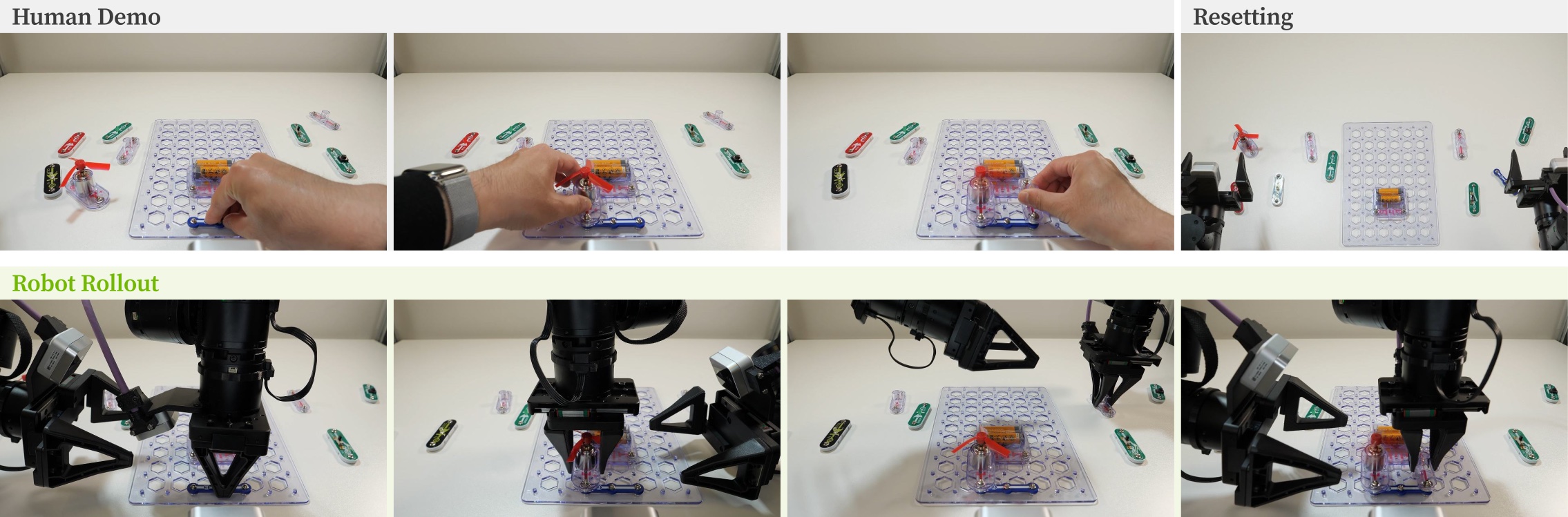
2. One-shot imitation from a single in-context human video. 6 / 10 on unseen circuit configurations; the matched baseline gets 0 / 10.

3. On-the-fly improvement, from DAgger data used differently. +36% over the same model without it.

4. Pretraining context length behaves like a scaling axis. Monotone from 128 to 8K timesteps, with no sign of saturation.

Why would a policy need memory?

A five-minute assembly task at 30 Hz is 9,000 control decisions.

Most robot foundation models see one of them:

  • Single observation: GR00T N1.7, \pi_0, \pi_{0.5}, OpenVLA, SmolVLA
  • A few consecutive frames, typically 2 to 8: RT-1, RT-2, Octo

Longer horizons get delegated upward, to keyframes or language. That answers what to do next, not fine visuomotor conditioning: which screw is already tightened, what the occluded part looked like two minutes ago.

The framing this paper borrows

Context length became a scaling axis for language models years ago. For robot policies it is still a fixed hyperparameter, usually set to 1.

And it is not free. Naively appending history can hurt: past actions leak into past observations, the policy latches onto them, and at inference it is temporally out of distribution.

The backbone: GR00T N1.7 in one slide

  • Eagle VLM encodes images and the language instruction into vision-language tokens \Phi_t
  • A Diffusion Transformer action head, 16 layers, 538M parameters, denoises an H-step action chunk with a flow-matching objective
  • Self-attention over the step’s own tokens, cross-attention into \Phi_t
  • Context: the current observation only

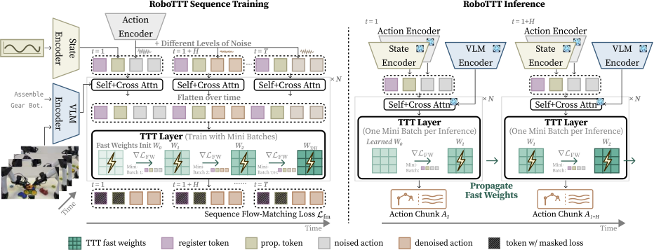
RoboTTT touches exactly one place: it inserts a TTT layer after the attention layers, in all 16 DiT blocks. 538M becomes 690M.

Figure 2: sequence training on the left, inference on the right. We walk through it properly in two slides.

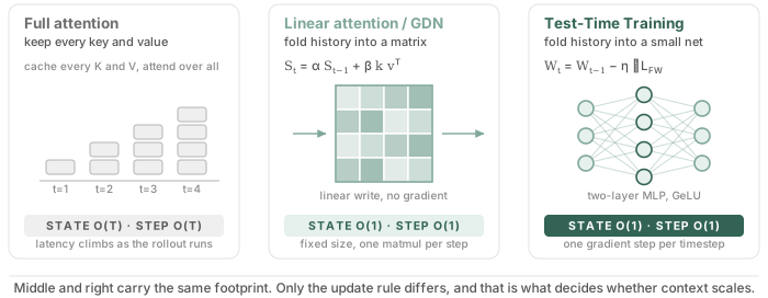
Memory, three shapes

From accumulation to overwriting

Linear attention (2020)

S_t = S_{t-1} + v_t k_t^{\top}

Pure accumulation. Write the same key twice and both writes stay in there, superposed.

DeltaNet (2021)

S_t = S_{t-1} + \beta_t\left(v_t - S_{t-1}k_t\right)k_t^{\top}

The delta rule: look up what is currently stored at k_t, and correct it toward v_t. Writing replaces instead of piling up.

Gated DeltaNet (2024)

Adds a learned decay so the state can also forget. Efficient chunked kernels made it practical at scale.

Why this slide exists

Gated DeltaNet is not background here. It is this paper’s control condition: same layer positions, same gating, same parameter count, only the update rule differs.

Every comparison later in the talk turns on that one substitution.

The spectrum, and where TTT sits

Sequence model Recurrent state How the state is written Cost / step State is… Init meta‑learned?
Full attention every key and value append k, v to the cache O(T) exact, unbounded –
LSTM a vector gated elementwise write O(1) low capacity no
Linear attention a matrix S S += v kT  (pure accumulation) O(1) a linear map no
DeltaNet a matrix S delta rule: overwrite what was stored at k O(1) a linear map no
Gated DeltaNet a matrix S delta rule + a learned forget gate O(1) a linear map no
Test-Time Training the weights W of a small MLP one gradient step on ‖fW(k) − v‖2 O(1) a nonlinear map yes

The two right-hand columns are the whole argument. Give TTT a linear fast model and one SGD step, and its update reduces algebraically to the delta rule: the same family as the row above. What breaks the equivalence is the nonlinearity, and the fact that the outer loss can meta-learn where the state starts.

Built for this talk; the paper states this in prose only.

Method

Update, then apply

RoboTTT · Mechanism

One timestep, up close: update then apply

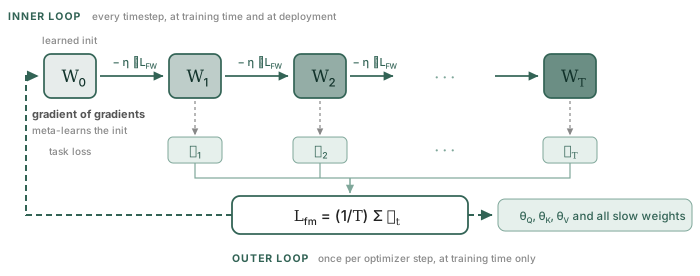
Inside a TTT layer the same small network is written to and then read from, once per timestep. Equations 1 and 2 are these five moves.

arrive

Built for this talk; the paper states this in prose only.

. . . . .

The two equations

Eq. 1   update W_t \leftarrow W_{t-1} - \eta\,\nabla_W \mathcal{L}_{\mathrm{FW}}\!\left(f_{W_{t-1}}(K_t),\, V_t\right)

Eq. 2   apply O_t = f_{W_t}(Q_t)

  • \mathcal{L}_{\mathrm{FW}}(\hat v, v) = \lVert \hat v - v \rVert^2
  • \eta is learned, on top of a constant base rate of 0.1
  • f_W is a two-layer MLP with GeLU, not a linear layer

\theta_Q, \theta_K, \theta_V and the initialisation W_0 are slow weights: learned by the outer task loss, frozen at inference.

W itself is a fast weight: it keeps moving after deployment.

Two loops, and the one that is easy to miss

What is being scaled

A robot trajectory is a stream of tuples: \xi = \left\{\left(o_t,\, q_t,\, A_t\right)\right\}_{t=1}^{T} \qquad\text{image, proprioception, action chunk}

A robot sequence model is a policy that conditions on the stream so far: \pi\left(A_t \mid \xi_{<t},\, o_t,\, q_t\right)

The quantity this paper scales is \lvert \xi_{<t} \rvert, the number of past timesteps the policy is conditioned on.

Not tokens. Not seconds. Control timesteps. Hold on to that; we come back to it at the end.

Inside one DiT block

RoboTTT · Model

Inside the diffusion transformer

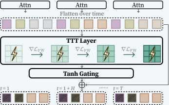
Follow the tokens through one block: attention runs within each chunk, then the TTT layer reads the flattened sequence in time order.

tokens

A simplified block view; the full architecture appears in the paper.

Animation reproduced verbatim from the official RoboTTT project page (NVIDIA GEAR), https://research.nvidia.com/labs/gear/robottt/

. . . . .

Three details that carry weight

1. TTT sits after attention. Attention handles within-step structure; TTT handles across-step structure. Clean division, and it is why the module ports to other backbones.

2. The VL tokens \Phi never enter the TTT path. Too expensive. Instead N = 16 learned register tokens per timestep attend to everything and carry the vision-language content across time.

3. The whole DiT input is one flat sequence. [\,R_1, \Phi_1, q_1, \tilde A_1,\; \ldots,\; R_T, \Phi_T, q_T, \tilde A_T\,]

Figure 2. Left: sequence training. Right: inference, fast weights propagating forward one timestep at a time.

Register tokens are doing real work here. The ablation shows they add +18% on top of TTT, and nothing at all when bolted onto GR00T without it.

Gating: how not to break the pretrained model

RoboTTT · Model

Tanh gating

A detail inside the DiT block: the update from the TTT layer passes through a learned tanh gate before it rejoins the residual stream.

sequence

A simplified view; the full gating figure appears in the paper.

Animation reproduced verbatim from the official RoboTTT project page (NVIDIA GEAR), https://research.nvidia.com/labs/gear/robottt/

. . . . .

Gating, in one line

Eq. 3 O = \tanh(\alpha) \odot O_{\mathrm{TTT}} + O_{\mathrm{attn}}

  • \alpha \in \mathbb{R}^d, learned per DiT layer
  • Initialised to 0.001, so \tanh(\alpha) \approx 0.001
  • At step zero the model is, numerically, still GR00T N1.7
  • The TTT path opens only as far as the loss asks it to

This is why RoboTTT can be initialised from base-model weights and pretrain only the new layers for 30K steps without destroying what GR00T already knew.

Figure 3. Flattened tokens go through the TTT layer, then the tanh gate, then rejoin the residual stream.

Sequence training: the outer loss

Eq. 4 \mathcal{L}_{\mathrm{fm}}(\xi; W_0) = \frac{1}{T}\sum_{t=1}^{T} \ell_t\!\left(\left(l, o_t, q_t, A_t\right);\, W_{t-1}\right)

  • One training example is a whole trajectory, or a contiguous sub-trajectory up to the context limit
  • Run TTT forward along it. At timestep t the policy is conditioned on W_{t-1}, the state the first t-1 steps produced
  • Average the per-step flow-matching loss, then take one optimiser step

Both things move on that step: the ordinary model weights, and W_0, through gradients of gradients. The initialisation is not chosen, it is learned, and it is learned to be a good starting point for robot trajectories specifically.

Sequence action forcing

Animation reproduced verbatim from the official RoboTTT project page (NVIDIA GEAR), https://research.nvidia.com/labs/gear/robottt/

. . . . .

The full training objective

Eq. 5 \mathcal{L}_{\mathrm{fm}}(\xi; W_0) = \frac{1}{T}\sum_{t=1}^{T} \mathbb{E}_{\tau_t, \epsilon}\left[\left\lVert v_\theta\!\left(\Phi_t, A_t^{\tau_t}, q_t;\, W_{t-1}\right) - \left(A_t - \epsilon\right) \right\rVert^2\right]

A_t^{\tau} = \tau A_t + (1-\tau)\,\epsilon, \qquad \epsilon \sim \mathcal{N}(\mathbf{0}, \mathbf{I})

\tau_t = s(1-u), \quad u \sim \mathrm{Beta}(1.5, 1), \quad s = 0.999

The subscript on \tau_t is the entire contribution. One noise level per timestep, drawn independently.

How much does it matter?

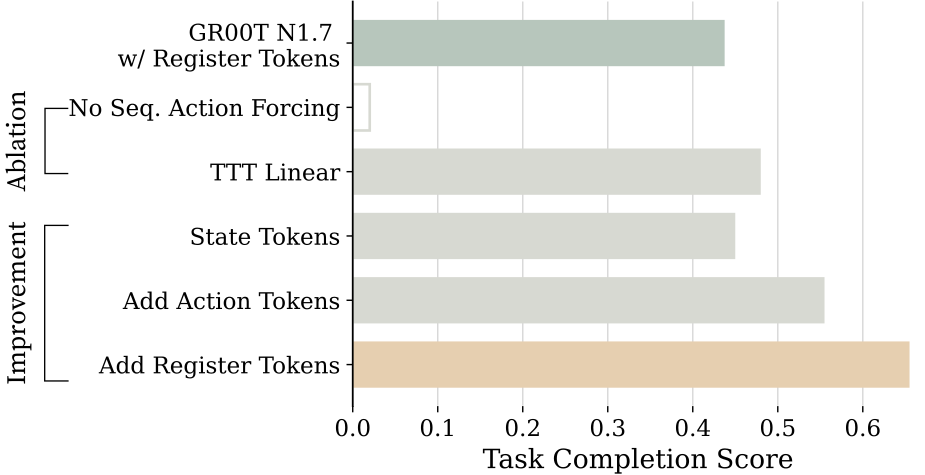
Removing sequence action forcing does not degrade the model gracefully. In the ablation the resulting motions are inaccurate enough that the robot makes no meaningful progress at all.

This is a load-bearing detail, not a tuning trick.

TBPTT: paying for context in time, not memory

Animation reproduced verbatim from the official RoboTTT project page (NVIDIA GEAR), https://research.nvidia.com/labs/gear/robottt/

. . . . . .

Loss masking: choosing what teaches and what only informs

Animation reproduced verbatim from the official RoboTTT project page (NVIDIA GEAR), https://research.nvidia.com/labs/gear/robottt/

. . . . . .

Implementation

Model

Backbone GR00T N1.7 (Eagle VLM + DiT)
TTT layers all 16 DiT layers
Fast model 2-layer MLP, GeLU
Inner LR learned, base 0.1
Positional RoPE, \theta = 10{,}000
Params 538M → 690M

Deployment

YAM bimanual, 4 × RealSense D405 at 480p, RTX 5090 @ 30 Hz

Training

Pretrain data tabletop bimanual + EgoScale egocentric human video
Pretrain 30K steps, 16 × GB200, new layers only
Post-train 20K steps, 8 × GB200, 1K context, all params
Optimiser AdamW, wd 1e-5
Schedule WSD peak 2e-5 / cosine peak 5e-5

Context is grown gradually during pretraining up to the target. Global batch drops from 64 to 16 above 4K context.

Experiments

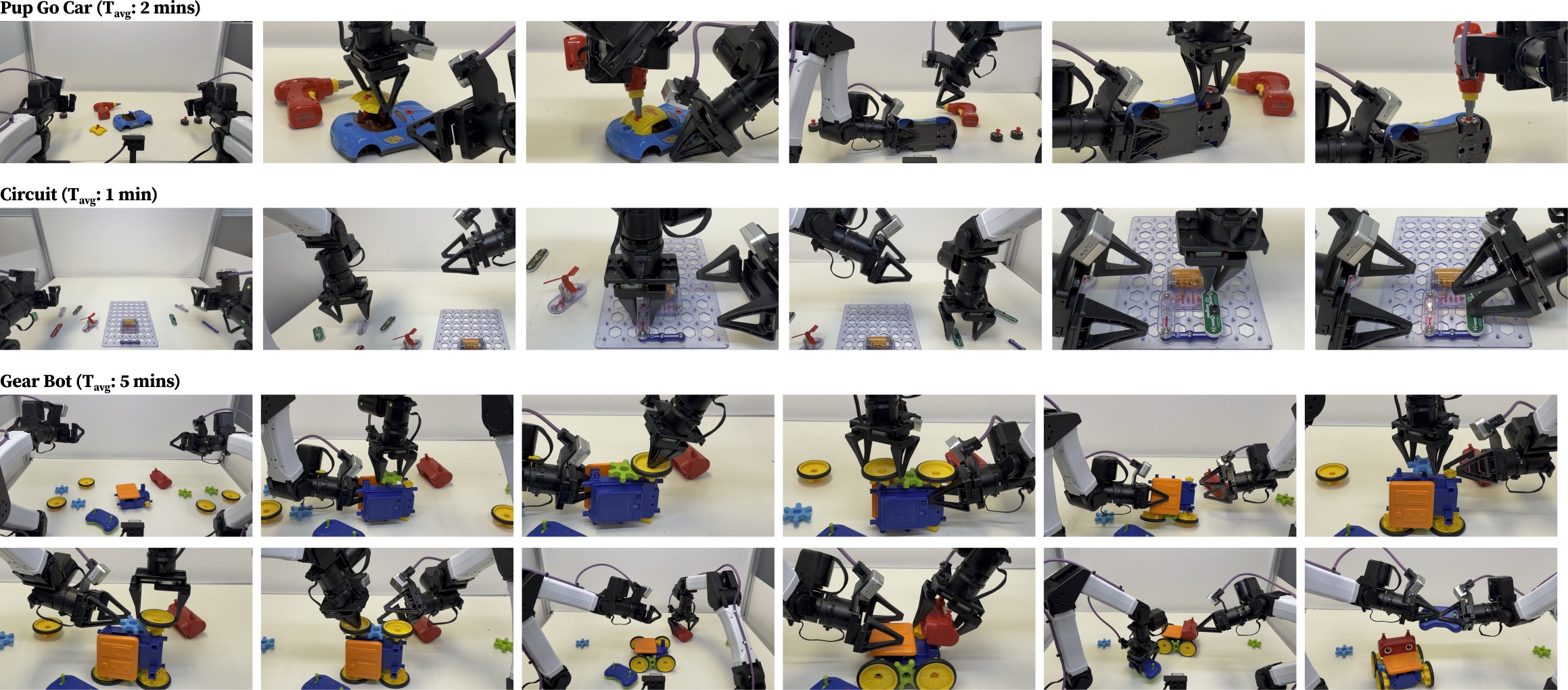
Three tasks, all bimanual, all long

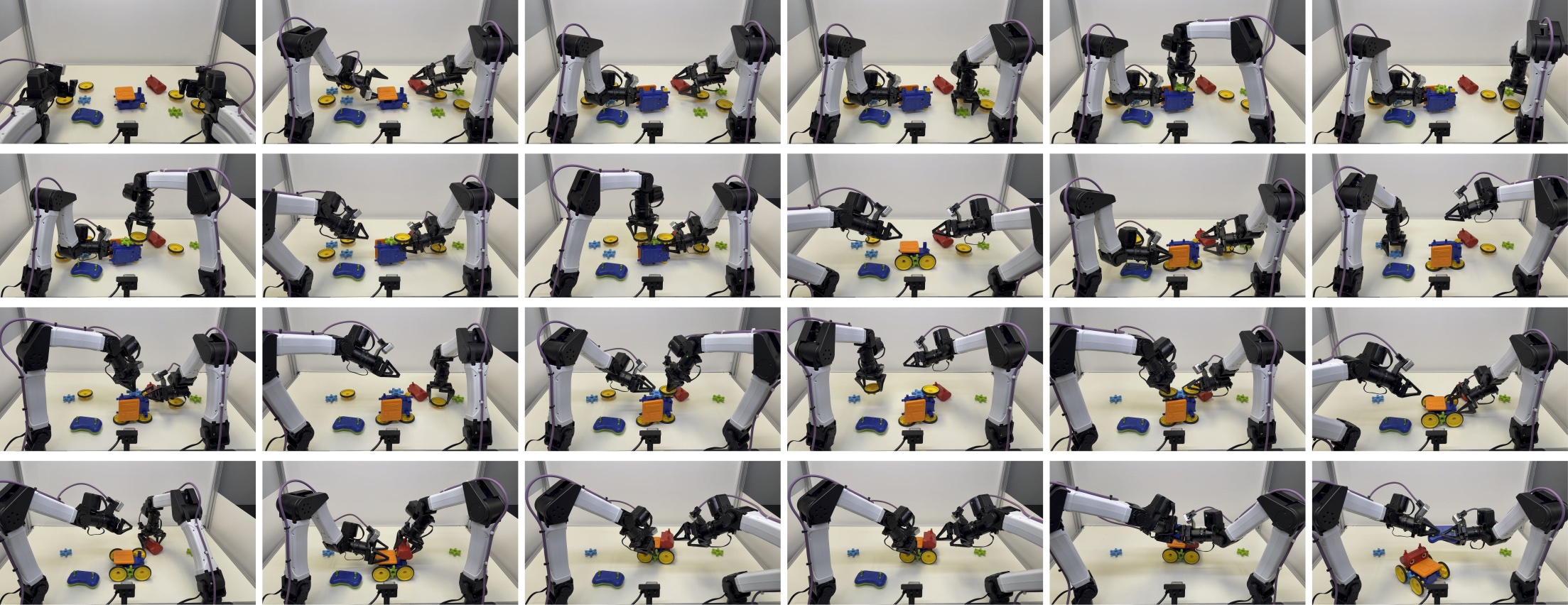
Pup Go Car · 8 h data, ~2 min/episode

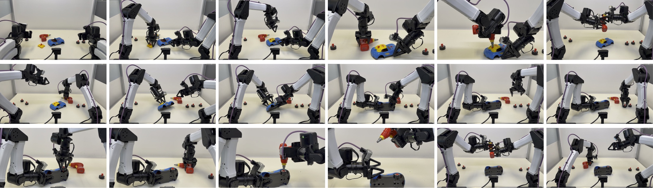
Roof, screw, drill, hand off the drill, flip the car, tire, drill again. 14 rubric stages.

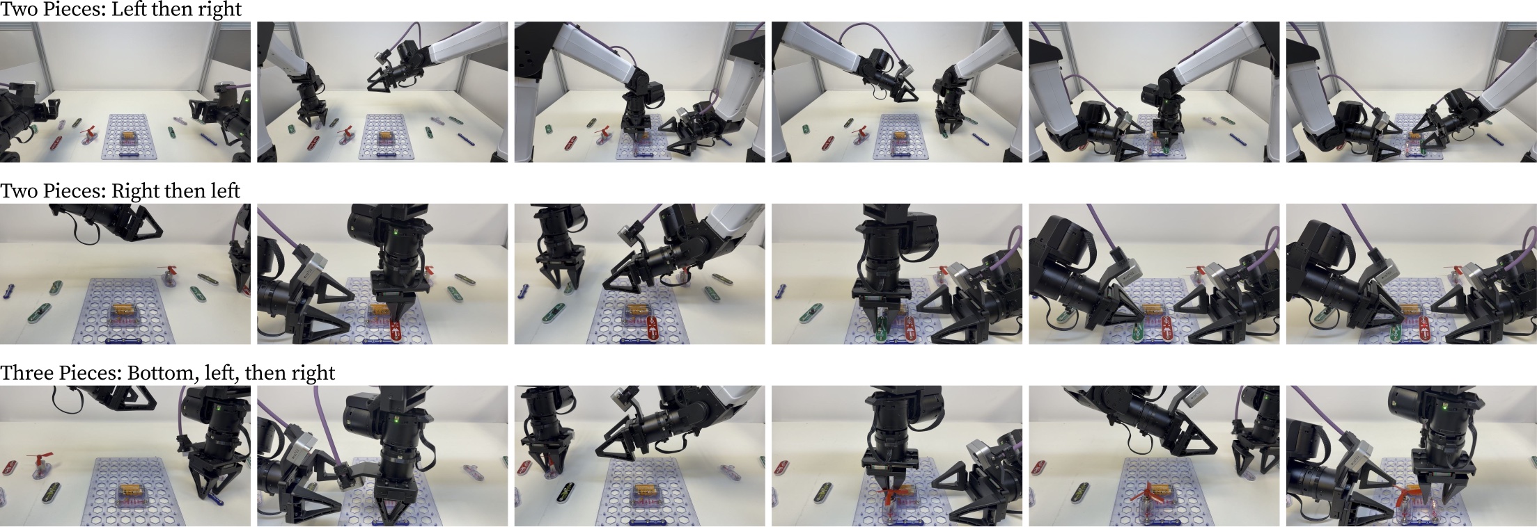
Circuit · 6 h data, ~1 min/episode

~80 configurations. Train on 20, test on the other 60. No partial credit if the order is wrong.

Gear Bot · 5 h data, ~5 min/episode

Gears and wheels on both sides, two chassis flips, head, then drive it with the remote. 10 stages.

What they look like at 1×

Pup Go Car

Circuit

Gear Bot

Real-time rollouts from the project page. Note the repeated, visually similar stages: this is exactly where a single-step policy loses track of where it is.

Baselines, and why the last one matters most

Baseline Context What it tests
GR00T N1.7 current observation the backbone, unmodified
GR00T N1.7 Hist. + 1 history frame does any history help?
Gated DeltaNet 1K timesteps does the update rule matter?

The GDN baseline replaces RoboTTT’s TTT layers with Gated DeltaNet layers and matches layer placement, gating, and parameter count. Same footprint, same plumbing, same amount of state. The only difference is how the state gets written.

Keep this in view: it turns a “our method wins” table into an actual experiment.

Protocol: 20 trials per task (10 for Gear Bot), identical recorded initial object placements across methods, a rubric-based completion score in [0,1] plus a count of fully successful trials.

Main results

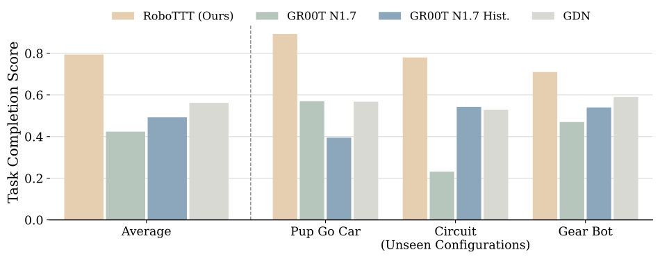
Figure 7. Rubric-based task completion score, averaged over the three tasks.

79%RoboTTT

56%GDN

42%GR00T

Fully successful trials (Table 1)

Pup Go Car Circuit Gear Bot
RoboTTT 9/20 13/20 2/10
GR00T N1.7 3/20 3/20 0/10
GR00T Hist. 0/20 8/20 0/10
GDN 3/20 8/20 0/10

Gear Bot is the headline: a five-minute, ten-stage assembly completed end to end, which no baseline ever does.
History, applied naively, is not free

On Pup Go Car:

57%GR00T, no history

39.5%GR00T + 1 frame

Adding a single history frame made the model worse, by a wide margin. Table 1 says the same thing more bluntly: 3/20 becomes 0/20.

Why

Past actions are implicitly encoded in past observations. A policy given both learns to read its own previous action off the frame instead of reading the scene. At inference it then drifts temporally out of distribution.

This is a known failure mode with its own literature, and it is the reason “just add history” was never the answer.

GDN improves on GR00T for Circuit and Gear Bot, but not for Pup Go Car either. Compressing history helps only if the compression is good enough.

The result the paper is really about

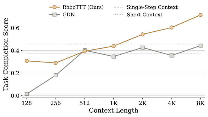
Figure 8. Pretraining context length from 128 to 8K timesteps, then post-train and evaluate closed-loop on all three tasks.

RoboTTT: 43.9% at 1K → 71.5% at 8K. +63% over its own 1K variant, +57% over the best short-context baseline. No sign of saturation.

GDN: no trend. Same footprint, same context lengths, same schedule.

The paper’s explanation, and it follows directly from the spectrum table: gradient descent has an initialisation and update dynamics that the outer loss can shape. Longer training sequences mean more update steps to shape them over. A linear associative state has nothing to meta-learn.

Below 1K it is weaker: 1K timesteps is half a minute, shorter than the shortest episode. Appendix A6.

One-shot imitation from a human video

The language prompt is “assemble circuit” for every configuration. The target is therefore identifiable only from the in-context video.

Score Successes
RoboTTT 65% 6/10
GDN 33% 0/10

GDN does not fail by a little. It picks up the wrong components, or assembles in the wrong order, ten times out of ten.

It encoded the video. It could not use it.

Perturbation robustness

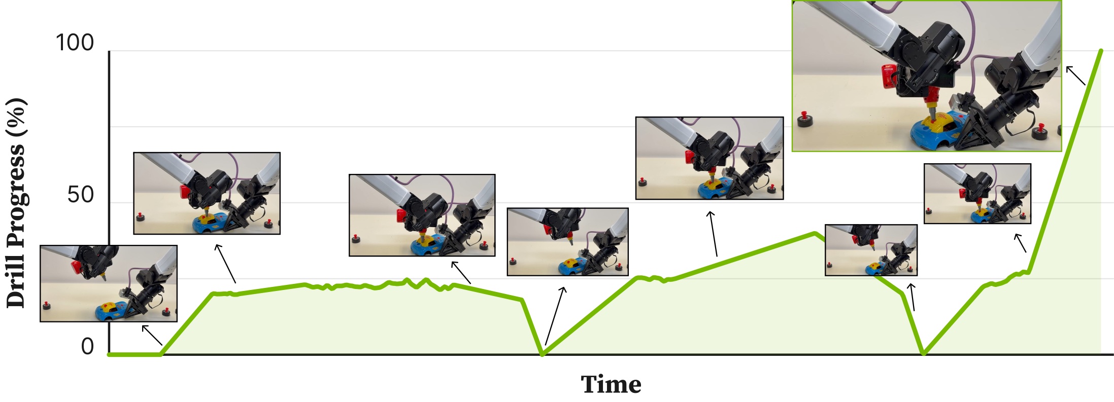
A human removes the roof after the robot has installed it. A policy that conditions on its own rollout should notice, go back, and reinstall it.

Roof Tire
RoboTTT 15/20 18/20
GDN 13/20 18/20
GR00T N1.7 10/20 11/20
GR00T Hist. 3/20 5/20

Worth saying plainly: this is where GDN is closest, and on tires it ties outright. 30 minutes of perturbation data was co-trained in, so every method has some of this.

On-the-fly improvement

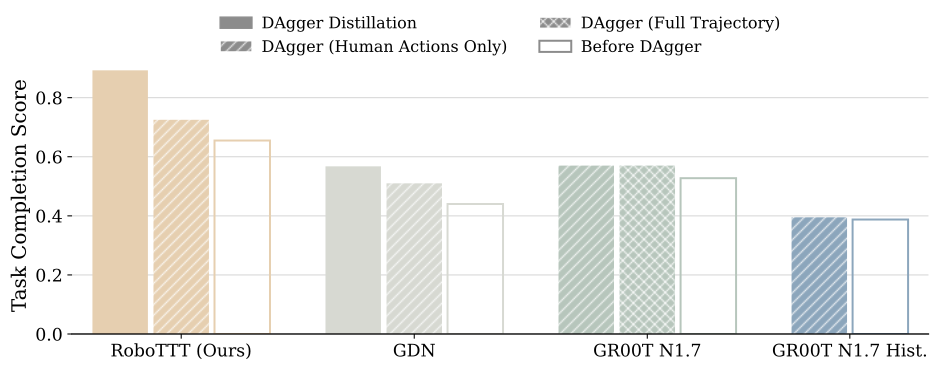
From the same 100 DAgger trajectories, 50 collected with RoboTTT as the base policy and 50 with GR00T:

  • Standard DAgger, corrections only: +13% on the sequence models
  • DAgger Distillation: +36% for RoboTTT, +29% for GDN

Fine-tuning GR00T on the full trajectories, suboptimal robot actions included, scores 57%. Identical to corrections alone.

The failures are worthless as targets. They are only valuable as context.

GDN gains 29% too, so this is not a TTT-specific trick. It applies to sequence-model policies generally, which makes it the most portable idea in the paper.

Reading the result

Limitations, as the authors state them

1. Scaling the training context costs training compute. Global batch drops from 64 to 16 above 4K. They point at TNT and similar techniques as the way out.

2. The inner objective is generic. \mathcal{L}_{\mathrm{FW}} is plain MSE reconstruction, inherited from the language-modelling literature. Nothing about it is robotics-specific, and they say so.

3. It does not fix every deployment failure. They name reinforcement learning, optimising task success directly, as the natural next step.

Also unexplored by their own admission: better test-time optimisers such as Muon, in place of plain gradient descent on the fast weights.

What the control condition actually shows

Gated DeltaNet and RoboTTT have the same state size, same gating, same layer placement, same parameter count. One substitution separates them.

Across the results, GDN behaves like this:

  • Perturbation recovery: nearly as good (13/20 and 18/20)
  • DAgger Distillation: benefits substantially (+29%)
  • One-shot imitation from video: 0 / 10
  • Context scaling: no trend at all

The pattern is not “GDN is worse”. It is GDN is fine until the task requires reaching back into the context for something specific.

The reading I would offer

Encoding a history and being able to use it are separate capabilities, and this pair of models isolates them about as cleanly as a real-robot experiment can.

A linear associative state accumulates; a gradient-updated nonlinear state is fit to the history, and its starting point can be meta-learned. Only the second gets better when you give it more context to be fit on.

Same reason the ablation shows TTT-Linear 27% worse than the MLP: as we saw, TTT-Linear is the delta rule.

Reading the numbers correctly

“8K context” means 8,000 control timesteps. At 30 Hz that is 4.4 minutes, not 8K tokens. The paper itself says “over four minutes” in one section and “about five minutes” in another. Worth stating precisely when you quote it.

“+87%” is a relative gain on a partial-credit rubric. 79% versus 42% on a [0,1] completion score. It is not a success rate. The success rates are 9/20, 13/20, 2/10, which is a different and more sobering picture, though still the best in the table by a clear margin.

10 to 20 trials, no error bars, no code or weights.

Be fair about this: a Gear Bot trial costs five minutes of real robot time, and initial placements were recorded and replayed per method. But individual cells are thin. The scaling curve is the robust result, because it is a trend across seven points rather than one comparison.

None of this makes the paper weaker. It makes the claim precise: a trend, established carefully, on one backbone and three tasks.

Three things to take away

1. The update rule decides whether context is worth scaling. Same state size, same cost, same plumbing. Gradient descent has an initialisation and dynamics that an outer loss can shape; a linear associative write does not.

2. Loss masking separates what conditions from what supervises. One small mechanism buys both one-shot imitation from human video and DAgger Distillation. And DAgger Distillation is not TTT-specific: it lifted the GDN baseline by 29% too.

3. Context length looks like a scaling axis for robot policies. 128 to 8K, monotone, no saturation. One backbone, three tasks, so: a well-supported hypothesis rather than a law. Someone should try to break it.


Thank you.

Paper: arXiv:2607.15275  ·  Project page and all videos: research.nvidia.com/labs/gear/robottt

Appendix

A1. Ablations

Two variants

  • No sequence action forcing: motions become inaccurate enough that the robot makes no meaningful progress
  • TTT-Linear instead of the MLP fast model: beats GR00T, but 27% worse than the MLP

The development roadmap

  • State tokens only → + action tokens: +23% (“aware of its past actions, the model better captures environment dynamics”)
  • → + register tokens: +18%
  • Register tokens added to GR00T alone: no help

A2. DAgger Distillation in detail

Data: 50 DAgger trajectories collected with RoboTTT as base policy + 50 with GR00T, pooled to 100 and used to train every method.

Method Gain
Standard DAgger, all four methods +9%
Standard DAgger, sequence models only +13%
DAgger Distillation, average +33%
  RoboTTT +36%
  GDN +29%

GR00T fine-tuned on full trajectories = GR00T fine-tuned on corrections only = 57%. Identical.

A3. Task rubrics

Pup Go Car, 14 graded stages:

0.05 roof picked up · 0.1 roof placed · 0.25 roof screw inserted · 0.3 drill picked up · 0.35 drill tip contacts screw · 0.45 roof screw tightened · 0.5 drill handed to right hand · 0.55 car flipped and stabilised · 0.6 tire picked up · 0.75 tire inserted · 0.8 drill picked up · 0.85 drill aligned to wheel screw · 0.9 wheel tightened · 1.0 drill handed to left hand

At most two attempts allowed for wheel assembly.

Gear Bot, additive: +0.1 per chassis flip, per gear or wheel installed, for the head, and for successfully using the remote.

Circuit, depends on the configuration:

  • 2 pieces, no switch: +0.5 each
  • 2 pieces with switch: +0.33 each, +0.33 to turn it on
  • 3 pieces, no switch: +0.33 each
  • 3 pieces with switch: +0.25 each, +0.25 to turn it on

No partial credit if the assembly order is wrong.

A4. Task definitions

A5. Training hyperparameters

Pretraining Post-training
GPUs 16 × GB200 8 × GB200
Steps 30K 20K
What is trained new sequence layers only (TTT or GDN) all parameters
Context grown gradually to target 1K
Per-device batch 4 (global 64) at ≤ 4K, 1 (global 16) above 1
Optimiser AdamW, weight decay 1e-5 AdamW, weight decay 1e-5
Schedule WSD, peak 2e-5 cosine, peak 5e-5

Data mixture: tabletop bimanual robot data plus EgoScale egocentric human video, curated to emphasise long trajectories.

A6. Why below 1K is weak

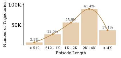
1K timesteps at 30 Hz is about half a minute, shorter than the shortest episode in any of the three tasks (Circuit averages 1 minute).

Two things go wrong at inference:

  1. The fast weights run past their training regime. They keep updating far beyond the number of steps ever seen during training, so the update dynamics the outer loss shaped no longer describe the regime the model is in.
  2. Positional embeddings extrapolate. RoPE positions extend to indices never observed in training.

Note what this implies for the scaling curve: part of the gain from 1K to 8K is matching the training context to the rollout horizon, not pure capacity. The curve keeps climbing past the point where the horizon is covered, which is what makes it a scaling result rather than a fix.

A7. The GDN baseline, precisely

Each TTT layer is replaced by a Gated DeltaNet layer from the Flash Linear Attention library, keeping layer placement, gating, and parameter count matched to RoboTTT.

\text{GDN:}\quad S_t = \alpha_t S_{t-1}\left(I - \beta_t k_t k_t^{\top}\right) + \beta_t v_t k_t^{\top}

\text{TTT-Linear:}\quad W_t = W_{t-1} - 2\eta\left(W_{t-1}k_t - v_t\right)k_t^{\top} = W_{t-1}\left(I - 2\eta\, k_t k_t^{\top}\right) + 2\eta\, v_t k_t^{\top}

With \alpha_t = 1 and \beta_t = 2\eta these are the same update. GDN adds a learned decay; TTT-MLP instead adds a nonlinearity and a meta-learned W_0.

That is the entire axis this paper’s comparison runs along.

A8. Full perturbation table and evaluation notes

Method Roof Tire
RoboTTT 15/20 18/20
GR00T N1.7 10/20 11/20
GR00T N1.7 Hist. 3/20 5/20
GDN 13/20 18/20

Aggregate: RoboTTT 33/40 = 83%, best short-context baseline 21/40 = 53%.

30 minutes of perturbation data was collected and co-trained with the task data, so all methods show some robustness.

Evaluation protocol

  • 20 rollouts for Pup Go Car and Circuit
  • 10 for Gear Bot, and 10 for the one-shot Circuit setting, because of evaluation time
  • Initial object placements recorded and reproduced identically across methods
  • Non-sequence baselines trained to a matched compute budget
  • Sequence models all post-trained at 1K context

Tire perturbation is the one place the GDN baseline ties RoboTTT outright. Worth conceding directly if it comes up.